Brain Tumor Image Classifier
Context
In this notebook, we will build an image classifier that can distinguish Pituitary Tumor from "No Tumor" MRI Scan images.
The dataset used in this notebook is available for download from Kaggle.
Although this dataset actually has a total of 3,264 images belonging to 4 classes - Glioma Tumor, Meningioma Tumor, Pituitary Tumor and No Tumor, for this project we have only taken two classes, and we are building a binary classification model to classify between the Pituitary Tumor category vs No Tumor.
For this project, we will only use 1000 of these images (830 training images and 170 Testing images). For the training dataset, we will take 395 MRI scans of No Tumor and 435 MRI scans of Pituitary Tumor. In our problem, we will also be using Data Augmentation to prevent overfitting, and to make our model model more generalised and robust.
We will use this to build an image classification model for this problem statement, and then show how we can improve our performance by simply "importing" a popular pre-trained model architecture and leveraging the idea of Transfer Learning.
Objectives
The objectives of this project are to:
- Load and understand the dataset
- Automatically label the images
- Perform Data Augmentation
- Build a classification model for this problem using CNNs
- Improve the model's performance through Transfer Learning
Importing Libraries
!pip install tensorflow
!pip install keras
# Library for creating data paths
import os
# Library for randomly selecting data points
import random
# Library for performing numerical computations
import numpy as np
# Library for creating and showing plots
import matplotlib.pyplot as plt
# Library for reading and showing images
import matplotlib.image as mpimg

# Importing sequential model type is used to build a simple linear stack of layers
from tensorflow.keras.models import Sequential, Model
# VGG16 is a pre-trained CNN model that is commonly used for image classification, we will use it for Transfer Learning
from tensorflow.keras.applications.vgg16 import VGG16
# For real-time data augmentation, which allows generating batches of tensor image data
from tensorflow.keras.preprocessing.image import ImageDataGenerator
# Importing utility functions for loading and converting images into arrays
from tensorflow.keras.preprocessing.image import img_to_array, load_img
# Importing different layers commonly used in building CNNs
from tensorflow.keras.layers import Conv2D, MaxPooling2D, Dense, Dropout, Flatten, BatchNormalization, Activation, LeakyReLU

# Importing optimizers
from tensorflow.keras.optimizers import Adam, SGD

# The below code can be used to ignore the warnings that may occur due to deprecations
import warnings
warnings.filterwarnings("ignore")
- Conv2D is used to create 2D convolutional layers, which help extract features from images.
- MaxPooling2D is used to reduce the spatial dimensions of the input, which helps in reducing the number of parameters and computation.
- Flatten is used to convert the multi-dimensional input into a single dimension for feeding into the dense layers.
- Dense layers are used to fully connect the neurons from the previous layer, typically for classification tasks.
- BatchNormalization helps to normalize the activations of the previous layer to speed up training and improve stability.
- Dropout is used as a regularization technique to prevent overfitting by randomly setting a fraction of input units to 0 during training.
Mounting the drive to load the dataset
from google.colab import drive
drive.mount('/content/drive')
Mounted at /content/drive
We have stored the images in a structured folder, and below we create the data paths to load images from those folders. This is required so that we can extract images in an auto-labelled fashion using Keras flow_from_directory.
# Parent directory where images are stored in drive
parent_dir = '/content/drive/My Drive/Texas McCombs/Computer Vision/brain-tumor-dataset'

# Path to the training and testing datasets within the parent directory
train_dir = os.path.join(parent_dir, 'Training')
validation_dir = os.path.join(parent_dir, 'Testing')

# Directory with our training images
train_pituitary_dir = os.path.join(train_dir, 'pituitary_tumor')
train_no_dir = os.path.join(train_dir, 'no_tumor')

# Directory with our testing images
validation_pituitary_dir = os.path.join(validation_dir, 'pituitary_tumor')
validation_no_dir = os.path.join(validation_dir, 'no_tumor')
Visualizing a few images
Before we move ahead and perform data augmentation, let's randomly check out some of the images and see what they look like:
# Create a list of image filenames from the directories
train_pituitary_file_names = os.listdir(train_pituitary_dir)
train_no_file_names = os.listdir(train_no_dir)

# Set up a figure for displaying the images in a grid format with 4 rows and 4 columns
fig = plt.figure(figsize=(16, 8))
fig.set_size_inches(16, 16)

# Generate the complete file paths for the first 8 images from each directory
pituitary_img_paths = [os.path.join(train_pituitary_dir, file_name) for file_name in train_pituitary_file_names[:8]]
no_img_paths = [os.path.join(train_no_dir, file_name) for file_name in train_no_file_names[:8]]

# Loop through the image paths and display them in the grid
for i, img_path in enumerate(pituitary_img_paths + no_img_paths):
    ax = plt.subplot(4, 4, i + 1)
    ax.axis('Off')

    img = mpimg.imread(img_path)  # Read the image from the path
    plt.imshow(img)  # Display the image on the subplot

# Show the plot with all images
plt.show()

As we can see, the images are quite different in size from each other.
This represents a problem, as most CNN architectures, including the pre-built model architectures that we will use for Transfer Learning, expect all the images to have the same size.
So we need to crop these images from the center to make sure they all have the same size. We can do this automatically while performing Data Augmentation, as shown below.
Data Augmentation
In most real-life case studies, it is generally difficult to collect lots of images and then train CNNs. In that case, one idea we can take advantage of is Data Augmentation. CNNs have the property of translational invariance, i.e., they can recognize an object as an object, even when its appearance varies translationally in some way. Taking this property into consideration, we can augment the images using the following techniques:
1. Horizontal Flip (should be set to True/False)
2. Vertical Flip (should be set to True/False)
3. Height Shift (should be between 0 and 1)
4. Width Shift (should be between 0 and 1)
5. Rotation (should be between 0 and 180)
6. Shear (should be between 0 and 1)
7. Zoom (should be between 0 and 1) etc.
We should not perform data augmentation in the validation/test data set.
Also, as mentioned above, we need to have images of the same size. So below,we resize the images by using the parameter target_size. Here we are resizing it to 224 x 224, as we will be using the VGG16 model for Transfer Learning, which takes image inputs as 224 x 224.
As this is a binary classification problem, we will need class labels. This is directly handled by the flow_from_directory function. It will take the images from the folder inside our specified directory, and the images from one folder will belong to same class.
As the train directory has 2 folders pituitary_tumor and no_tumor, it will read the directory and each folder will be considered a separate class. We specify class_model = 'binary' as this is a binary classification problem.
As the folders inside the directory will be read in an alphabetical order, the no_tumor folder will be given a label 0, and pituitary_tumor will be label 1.
# All images to be rescaled by 1/255. Train images go through the data augmentation.
train_datagen = ImageDataGenerator(rescale=1. / 255.0,
                              horizontal_flip = True,
                              vertical_flip = False,
                              height_shift_range= 0.1,
                              width_shift_range=0.1,
                              rotation_range=20,
                              shear_range = 0.1,
                              zoom_range=0.1)

# Only perform image scaling but no data augmentation for the test images.
test_datagen  = ImageDataGenerator(rescale = 1.0/255.)

# Flowing training images in batches of 20 using train_datagen generator
train_generator = train_datagen.flow_from_directory(train_dir,
                                                    batch_size=20,
                                                    class_mode='binary',
                                                    target_size=(224, 224))

# Flowing testing images in batches of 20 using test_datagen generator
validation_generator =  test_datagen.flow_from_directory(validation_dir,
                                                         batch_size=20,
                                                         class_mode='binary',
                                                         target_size=(224, 224))
Found 830 images belonging to 2 classes.
Found 170 images belonging to 2 classes.
Let's look at some examples of our augmented training data.
This is helpful for understanding the extent to which data is being manipulated prior to training, and can be compared with how the raw data looks prior to data augmentation.
# Fetch the next batch of images and labels from the training data generator
images, labels = next(train_generator)

# Create a 4x4 grid of subplots to display the images
fig, axes = plt.subplots(4, 4, figsize = (16, 8))
# Set the size of the figure for better visibility
fig.set_size_inches(16, 16)

# Loop through each image, label, and subplot axis to display the images and titles
for (image, label, ax) in zip(images, labels, axes.flatten()):
    ax.imshow(image)
    if label == 1:
        ax.set_title('pituitary tumor')
    else:
        ax.set_title('no tumor')
    ax.axis('off')   # Hide the axis lines and labels for better image presentation

CNN Model Building
Once the data is augmented and cropped to have the same size, we are now ready to build a first baseline CNN model to classify no_tumor vs pituitary_tumor.
When building our custom model, we have used Batch Normalization and Dropout layers as regularization techniques to prevent overfitting.
# Initialize a Sequential model, which allows adding layers in a linear stack
cnn_model = Sequential()

# Add a 2D convolutional layer with 64 filters, a 3x3 kernel, ReLU activation, and input shape of 224x224x3 (RGB image)
cnn_model.add(Conv2D(64, (3,3), activation='relu', input_shape=(224, 224, 3), padding='same'))

# Add a MaxPooling layer to reduce spatial dimensions by 2x2 (downsampling)
cnn_model.add(MaxPooling2D(2,2))

# Add BatchNormalization to normalize the activations and improve training stability
cnn_model.add(BatchNormalization())

# Add another 2D convolutional layer with 32 filters and ReLU activation
cnn_model.add(Conv2D(32, (3,3), activation='relu', padding='same'))

# Add another MaxPooling layer for further downsampling
cnn_model.add(MaxPooling2D(2,2))

# Add BatchNormalization again to stabilize and improve training
cnn_model.add(BatchNormalization())

# Add another 2D convolutional layer with 32 filters
cnn_model.add(Conv2D(32, (3,3), activation='relu', padding='same'))

# Add another MaxPooling layer for spatial dimension reduction
cnn_model.add(MaxPooling2D(2,2))

# Add a final 2D convolutional layer with 16 filters
cnn_model.add(Conv2D(16, (3,3), activation='relu', padding='same'))

# Flatten the multi-dimensional output from the convolutional layers to feed it into fully connected layers
cnn_model.add(Flatten())

# Add a fully connected Dense layer with 64 units and ReLU activation
cnn_model.add(Dense(64, activation='relu'))

# Add a Dropout layer to prevent overfitting by randomly dropping 25% of the neurons during training
cnn_model.add(Dropout(0.25))

# Add another fully connected Dense layer with 32 units and ReLU activation
cnn_model.add(Dense(32, activation='relu'))

# Add another Dropout layer with 25% dropout rate
cnn_model.add(Dropout(0.25))

# Add a third Dense layer with 32 units and ReLU activation
cnn_model.add(Dense(32, activation='relu'))

# Add the final output layer with a single neuron and sigmoid activation (for binary classification)
cnn_model.add(Dense(1, activation='sigmoid'))
# Compile the CNN model by specifying the loss function, optimizer, and evaluation metrics
# "binary_crossentropy" is used for binary classification (2 classes)
# "adam" is an optimizer that adjusts the learning rate based on the gradients
# "accuracy" is used as a metric to evaluate the model's performance during training
cnn_model.compile(loss="binary_crossentropy", optimizer="adam", metrics=['accuracy'])

# Display the summary of the CNN model, which shows the layer details, number of parameters, and model architecture
cnn_model.summary()
Model: "sequential"
_________________________________________________________________
 Layer (type)                Output Shape              Param #
=================================================================
 conv2d (Conv2D)             (None, 224, 224, 64)      1792

 max_pooling2d (MaxPooling2  (None, 112, 112, 64)      0
 D)

 batch_normalization (Batch  (None, 112, 112, 64)      256
 Normalization)

 conv2d_1 (Conv2D)           (None, 112, 112, 32)      18464

 max_pooling2d_1 (MaxPoolin  (None, 56, 56, 32)        0
 g2D)

 batch_normalization_1 (Bat  (None, 56, 56, 32)        128
 chNormalization)

 conv2d_2 (Conv2D)           (None, 56, 56, 32)        9248

 max_pooling2d_2 (MaxPoolin  (None, 28, 28, 32)        0
 g2D)

 conv2d_3 (Conv2D)           (None, 28, 28, 16)        4624

 flatten (Flatten)           (None, 12544)             0

 dense (Dense)               (None, 64)                802880

 dropout (Dropout)           (None, 64)                0

 dense_1 (Dense)             (None, 32)                2080

 dropout_1 (Dropout)         (None, 32)                0

 dense_2 (Dense)             (None, 32)                1056

 dense_3 (Dense)             (None, 1)                 33

=================================================================
Total params: 840561 (3.21 MB)
Trainable params: 840369 (3.21 MB)
Non-trainable params: 192 (768.00 Byte)
_________________________________________________________________
# Pulling a single large batch of random testing data for testing after each epoch
testX, testY = validation_generator.next()
# Fit the CNN model using specified configuration
model_history = cnn_model.fit(train_generator,
                              validation_data=(testX, testY),
                              epochs=10)
Epoch 1/10
42/42 [==============================] - 142s 3s/step - loss: 0.6342 - accuracy: 0.7325 - val_loss: 0.6587 - val_accuracy: 0.4500
Epoch 2/10
42/42 [==============================] - 95s 2s/step - loss: 0.3805 - accuracy: 0.8470 - val_loss: 1.2365 - val_accuracy: 0.4500
Epoch 3/10
42/42 [==============================] - 94s 2s/step - loss: 0.2949 - accuracy: 0.8699 - val_loss: 1.5326 - val_accuracy: 0.3500
Epoch 4/10
42/42 [==============================] - 95s 2s/step - loss: 0.2716 - accuracy: 0.9120 - val_loss: 3.0359 - val_accuracy: 0.3500
Epoch 5/10
42/42 [==============================] - 97s 2s/step - loss: 0.2594 - accuracy: 0.8964 - val_loss: 4.0897 - val_accuracy: 0.3500
Epoch 6/10
42/42 [==============================] - 95s 2s/step - loss: 0.1802 - accuracy: 0.9349 - val_loss: 1.7176 - val_accuracy: 0.3500
Epoch 7/10
42/42 [==============================] - 95s 2s/step - loss: 0.1293 - accuracy: 0.9554 - val_loss: 1.1518 - val_accuracy: 0.5500
Epoch 8/10
42/42 [==============================] - 94s 2s/step - loss: 0.1701 - accuracy: 0.9386 - val_loss: 0.4393 - val_accuracy: 0.7000
Epoch 9/10
42/42 [==============================] - 95s 2s/step - loss: 0.1488 - accuracy: 0.9470 - val_loss: 0.4006 - val_accuracy: 0.8500
Epoch 10/10
42/42 [==============================] - 93s 2s/step - loss: 0.1226 - accuracy: 0.9639 - val_loss: 1.1330 - val_accuracy: 0.6500
# Evaluating on the Test dataset
cnn_model.evaluate(validation_generator)
9/9 [==============================] - 39s 5s/step - loss: 0.9733 - accuracy: 0.7059
[0.9733238816261292, 0.7058823704719543]
Findings
- Our model had 840,369 trainable parameters.
- After running 10 epochs, we were able to achieve a training accuracy of ~95% and a testing accuracy of ~72%.
- Even after using Data Augmentation, Batch Normalization and the Dropout Layers, the model seems to have highly overfit on the training dataset and is performing somewhat poorly.
Model Building using Transfer Learning: VGG 16
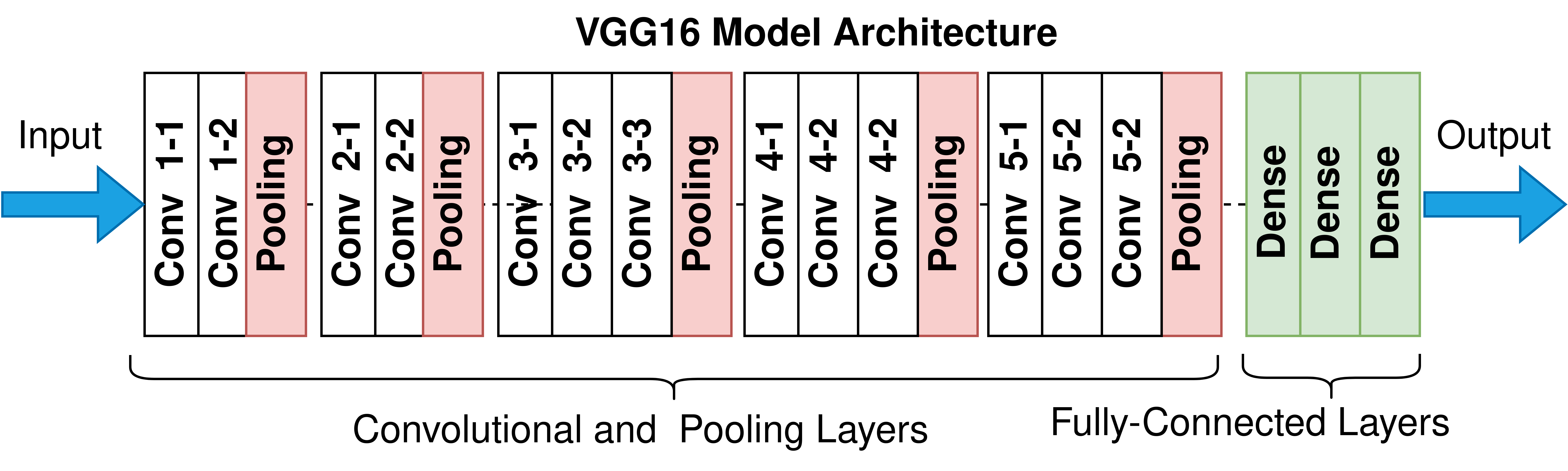
Now, let's try again, but this time, using the idea of Transfer Learning. We will be loading a pre-built architecture - VGG16, which was trained on the ImageNet dataset and finished runner-up in the ImageNet competition in 2014. Below is a schematic of the VGG16 model.
For training VGG16, we will directly use the convolutional and pooling layers and freeze their weights i.e. no training will be done on them. We will remove the already-present fully-connected layers and add our own fully-connected layers for this binary classification task.
# Summary of the whole VGG 16 model
model = VGG16(weights='imagenet')
model.summary()
Downloading data from https://storage.googleapis.com/tensorflow/keras-applications/vgg16/vgg16_weights_tf_dim_ordering_tf_kernels.h5
553467096/553467096 [==============================] - 2s 0us/step
Model: "vgg16"
_________________________________________________________________
 Layer (type)                Output Shape              Param #
=================================================================
 input_1 (InputLayer)        [(None, 224, 224, 3)]     0

 block1_conv1 (Conv2D)       (None, 224, 224, 64)      1792

 block1_conv2 (Conv2D)       (None, 224, 224, 64)      36928

 block1_pool (MaxPooling2D)  (None, 112, 112, 64)      0

 block2_conv1 (Conv2D)       (None, 112, 112, 128)     73856

 block2_conv2 (Conv2D)       (None, 112, 112, 128)     147584

 block2_pool (MaxPooling2D)  (None, 56, 56, 128)       0

 block3_conv1 (Conv2D)       (None, 56, 56, 256)       295168

 block3_conv2 (Conv2D)       (None, 56, 56, 256)       590080

 block3_conv3 (Conv2D)       (None, 56, 56, 256)       590080

 block3_pool (MaxPooling2D)  (None, 28, 28, 256)       0

 block4_conv1 (Conv2D)       (None, 28, 28, 512)       1180160

 block4_conv2 (Conv2D)       (None, 28, 28, 512)       2359808

 block4_conv3 (Conv2D)       (None, 28, 28, 512)       2359808

 block4_pool (MaxPooling2D)  (None, 14, 14, 512)       0

 block5_conv1 (Conv2D)       (None, 14, 14, 512)       2359808

 block5_conv2 (Conv2D)       (None, 14, 14, 512)       2359808

 block5_conv3 (Conv2D)       (None, 14, 14, 512)       2359808

 block5_pool (MaxPooling2D)  (None, 7, 7, 512)         0

 flatten (Flatten)           (None, 25088)             0

 fc1 (Dense)                 (None, 4096)              102764544

 fc2 (Dense)                 (None, 4096)              16781312

 predictions (Dense)         (None, 1000)              4097000

=================================================================
Total params: 138357544 (527.79 MB)
Trainable params: 138357544 (527.79 MB)
Non-trainable params: 0 (0.00 Byte)
_________________________________________________________________
Creating a new model out of the pre-trained VGG 16 model:
# Get the output of the specific layer ('block5_pool') from the pre-trained VGG model for transfer learning
# 'block5_pool' is the last pooling layer of the VGG16 model, which helps capture higher-level features
transfer_layer = model.get_layer('block5_pool')

# Create a new model that uses the input of the original model but outputs the feature map from the 'block5_pool' layer
# This is done to use the VGG16 model for feature extraction, as part of transfer learning
vgg_model = Model(inputs=model.input, outputs=transfer_layer.output)
# Display the architecture of the new model
vgg_model.summary()
Model: "model"
_________________________________________________________________
 Layer (type)                Output Shape              Param #
=================================================================
 input_1 (InputLayer)        [(None, 224, 224, 3)]     0

 block1_conv1 (Conv2D)       (None, 224, 224, 64)      1792

 block1_conv2 (Conv2D)       (None, 224, 224, 64)      36928

 block1_pool (MaxPooling2D)  (None, 112, 112, 64)      0

 block2_conv1 (Conv2D)       (None, 112, 112, 128)     73856

 block2_conv2 (Conv2D)       (None, 112, 112, 128)     147584

 block2_pool (MaxPooling2D)  (None, 56, 56, 128)       0

 block3_conv1 (Conv2D)       (None, 56, 56, 256)       295168

 block3_conv2 (Conv2D)       (None, 56, 56, 256)       590080

 block3_conv3 (Conv2D)       (None, 56, 56, 256)       590080

 block3_pool (MaxPooling2D)  (None, 28, 28, 256)       0

 block4_conv1 (Conv2D)       (None, 28, 28, 512)       1180160

 block4_conv2 (Conv2D)       (None, 28, 28, 512)       2359808

 block4_conv3 (Conv2D)       (None, 28, 28, 512)       2359808

 block4_pool (MaxPooling2D)  (None, 14, 14, 512)       0

 block5_conv1 (Conv2D)       (None, 14, 14, 512)       2359808

 block5_conv2 (Conv2D)       (None, 14, 14, 512)       2359808

 block5_conv3 (Conv2D)       (None, 14, 14, 512)       2359808

 block5_pool (MaxPooling2D)  (None, 7, 7, 512)         0

=================================================================
Total params: 14714688 (56.13 MB)
Trainable params: 14714688 (56.13 MB)
Non-trainable params: 0 (0.00 Byte)
_________________________________________________________________
Another way of creating a new model out of the VGG 16 model (Recommended):
To remove the fully-connected layers of the imported pre-trained model, while calling it from Keras we can also specify an additonal keyword argument that is include_top.
If we specify include_top = False, then the model will be imported without the fully-connected layers. Here we won't have to do the above steps of getting the last convolutional layer and creating a separate model.
If we are specifying include_top = False, we will also have to specify our input image shape.
Keras has this keyword argument as generally while importing a pre-trained CNN model, we don't require the fully-connected layers and we train our own fully-connected layers for our task.
# Create a new model that uses the pre-trained weights from the ImageNet dataset,
# exclude the fully connected layers (top layers) of the VGG16 model, leaving just the convolutional layers,
# and use specified input image size and the number of color channels (RGB)
vgg_model = VGG16(weights='imagenet', include_top=False, input_shape=(224,224,3))

# Display the architecture of the new model
vgg_model.summary()
Downloading data from https://storage.googleapis.com/tensorflow/keras-applications/vgg16/vgg16_weights_tf_dim_ordering_tf_kernels_notop.h5
58889256/58889256 [==============================] - 0s 0us/step
Model: "vgg16"
_________________________________________________________________
 Layer (type)                Output Shape              Param #
=================================================================
 input_2 (InputLayer)        [(None, 224, 224, 3)]     0

 block1_conv1 (Conv2D)       (None, 224, 224, 64)      1792

 block1_conv2 (Conv2D)       (None, 224, 224, 64)      36928

 block1_pool (MaxPooling2D)  (None, 112, 112, 64)      0

 block2_conv1 (Conv2D)       (None, 112, 112, 128)     73856

 block2_conv2 (Conv2D)       (None, 112, 112, 128)     147584

 block2_pool (MaxPooling2D)  (None, 56, 56, 128)       0

 block3_conv1 (Conv2D)       (None, 56, 56, 256)       295168

 block3_conv2 (Conv2D)       (None, 56, 56, 256)       590080

 block3_conv3 (Conv2D)       (None, 56, 56, 256)       590080

 block3_pool (MaxPooling2D)  (None, 28, 28, 256)       0

 block4_conv1 (Conv2D)       (None, 28, 28, 512)       1180160

 block4_conv2 (Conv2D)       (None, 28, 28, 512)       2359808

 block4_conv3 (Conv2D)       (None, 28, 28, 512)       2359808

 block4_pool (MaxPooling2D)  (None, 14, 14, 512)       0

 block5_conv1 (Conv2D)       (None, 14, 14, 512)       2359808

 block5_conv2 (Conv2D)       (None, 14, 14, 512)       2359808

 block5_conv3 (Conv2D)       (None, 14, 14, 512)       2359808

 block5_pool (MaxPooling2D)  (None, 7, 7, 512)         0

=================================================================
Total params: 14714688 (56.13 MB)
Trainable params: 14714688 (56.13 MB)
Non-trainable params: 0 (0.00 Byte)
_________________________________________________________________
We are 'freezing' the pre-trained model layers next:
# Making all the layers of the VGG model non-trainable. i.e. freezing them
for layer in vgg_model.layers:
    layer.trainable = False
# Print the frozen layers in the model
for layer in vgg_model.layers:
    print(layer.name, layer.trainable)
input_2 False
block1_conv1 False
block1_conv2 False
block1_pool False
block2_conv1 False
block2_conv2 False
block2_pool False
block3_conv1 False
block3_conv2 False
block3_conv3 False
block3_pool False
block4_conv1 False
block4_conv2 False
block4_conv3 False
block4_pool False
block5_conv1 False
block5_conv2 False
block5_conv3 False
block5_pool False
Create our final model:
# Initialize a Sequential model, which allows adding layers in a linear stack
new_model = Sequential()

# Adding the convolutional part of the VGG16 model from above
new_model.add(vgg_model)

# Flattening the output of the VGG16 model because it is from a convolutional layer
new_model.add(Flatten())

# Add two fully connected Dense layers with 32 units and ReLU activation
new_model.add(Dense(32, activation='relu'))
new_model.add(Dense(32, activation='relu'))

# Add the final output layer with a single neuron and sigmoid activation (for binary classification)
new_model.add(Dense(1, activation='sigmoid'))
# Compile our new model by specifying the loss function, optimizer, and evaluation metrics
# "adam" is an optimizer that adjusts the learning rate based on the gradients
# "accuracy" is used as a metric to evaluate the model's performance during training
new_model.compile(optimizer='adam', loss='binary_crossentropy', metrics=['accuracy'])

# Display the summary of our new model, which shows the layer details, number of parameters, and model architecture
new_model.summary()
Model: "sequential_2"
_________________________________________________________________
 Layer (type)                Output Shape              Param #
=================================================================
 vgg16 (Functional)          (None, 7, 7, 512)         14714688

 flatten_2 (Flatten)         (None, 25088)             0

 dense_7 (Dense)             (None, 32)                802848

 dense_8 (Dense)             (None, 32)                1056

 dense_9 (Dense)             (None, 1)                 33

=================================================================
Total params: 15518625 (59.20 MB)
Trainable params: 803937 (3.07 MB)
Non-trainable params: 14714688 (56.13 MB)
_________________________________________________________________
# Fit the VGG model using specified configuration
new_model_history = new_model.fit(train_generator,
                                  validation_data=(testX, testY),
                                  epochs=5)
Epoch 1/5
42/42 [==============================] - 206s 5s/step - loss: 0.4778 - accuracy: 0.7699 - val_loss: 0.3343 - val_accuracy: 0.9000
Epoch 2/5
42/42 [==============================] - 203s 5s/step - loss: 0.1036 - accuracy: 0.9639 - val_loss: 0.3332 - val_accuracy: 0.8500
Epoch 3/5
42/42 [==============================] - 202s 5s/step - loss: 0.0765 - accuracy: 0.9807 - val_loss: 0.2811 - val_accuracy: 0.9000
Epoch 4/5
42/42 [==============================] - 202s 5s/step - loss: 0.0694 - accuracy: 0.9759 - val_loss: 0.3008 - val_accuracy: 0.9000
Epoch 5/5
42/42 [==============================] - 203s 5s/step - loss: 0.0433 - accuracy: 0.9867 - val_loss: 0.1710 - val_accuracy: 0.9000
# Evaluating on the Test set
new_model.evaluate(validation_generator)
9/9 [==============================] - 40s 4s/step - loss: 0.2322 - accuracy: 0.8765
[0.23218101263046265, 0.8764705657958984]
# Create a function to plot loss and val_loss graphs
def plot_history(history):
    N = len(history.history["accuracy"])
    plt.figure()
    plt.plot(np.arange(0, N), history.history["accuracy"], label="train_accuracy")
    plt.plot(np.arange(0, N), history.history["val_accuracy"], label="val_accuracy")
    plt.title("Training accuracy Dataset")
    plt.xlabel("Epoch #")
    plt.ylabel("accuracy")
    plt.legend(loc="upper right")
# Plotting the loss vs epoch curve for the basic CNN model without Transfer Learning
plot_history(model_history)

- The graph above illustrates the training accuracy and validation accuracy at each epoch for our CNN model.
- A significant gap is observed between the training accuracy and validation accuracy scores throughout the training process, indicating that the model is overfitting to the training data.
- Overall, the average validation accuracy remains unsatisfactory, suggesting that the model may not generalize well to unseen data.
# Plotting the loss vs epoch curve for the Transfer Learning model
plot_history(new_model_history)

- The graph above shows the training accuracy and validation accuracy at each epoch for the VGG model.
- A sharp increase in the training accuracy is observed early in the training, with the model reaching a high score quickly. Similarly, the validation accuracy improves significantly, indicating that the model is learning effectively.
- Unlike the previous graph, there seems to be less overfitting, as the validation accuracy maintains a steady upward trajectory, closely following the training accuracy.
- Overall, the score improvements demonstrate promising results, and the model seems to be generalizing better with fewer signs of overfitting.
Findings
- Our model has 803,937 Trainable parameters.
- After running only 5 epochs we were able to achieve a training accuracy of ~98% and a validation accuracy of ~ 91%.
Conclusions
The difference in both models is evident. Both models had nearly the same number of trainable parameters. However even after training the custom CNN model for 10 epochs, it could not attain accuracies as high as we achieved with Transfer Learning.
The Transfer Learning model has converged faster than the custom CNN model in only 5 epochs.
That's a good level of improvement just by directly using a pre-trained architecture such as VGG16.
This model can, in fact, further be tuned to achieve the accuracies required for practical applicability in the medical domain.